Data Science with Python Full Course 2026: Foundation to Expert in 21 Free Sessions by ABC Trainings (Updated August 2026)
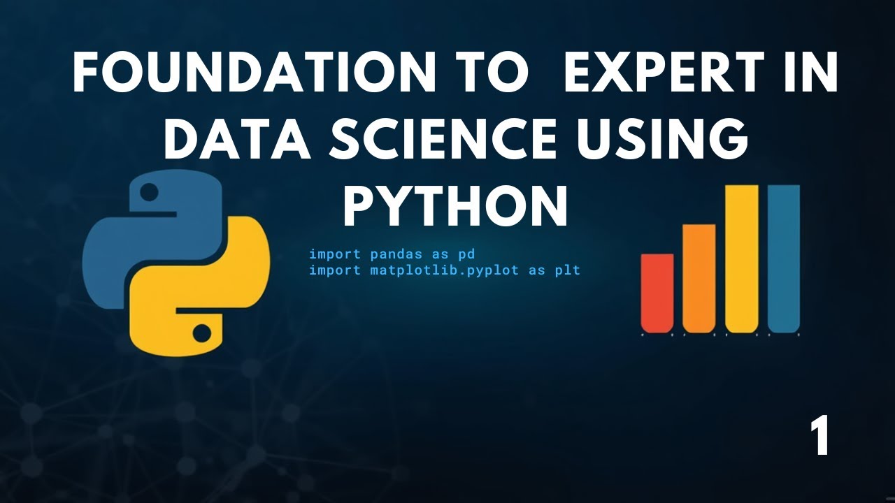
Data science is the role that every company now needs and almost no one can fill well. NASSCOM estimates India will need 250,000 additional data professionals by 2027, while fresher salaries for data analysts with Python skills have climbed past Rs 5.5 lakh per annum in Pune and Rs 6.8 lakh in Bengaluru in 2025. What is driving this? The answer is simple: businesses generate more data than ever before -- from e-commerce purchases and logistics sensors to hospital EMR systems and factory IoT devices -- and they need people who can process that data into decisions. Python is the language for this work. More than 76 percent of data scientists globally use Python as their primary tool (Stack Overflow Survey 2024), and every major data library -- NumPy, Pandas, scikit-learn, TensorFlow, Keras -- is Python-first. This guide covers all 21 sessions of ABC Trainings' Foundation to Expert in Data Science Using Python, a free YouTube series that takes you from understanding what data science means through hands-on machine learning and NLP projects. You can follow along in Jupyter Notebook with no software cost.
- Python is the industry standard for data science -- 76% of practitioners use it as their primary tool
- 21 sessions cover: Python foundations, NumPy/Pandas, descriptive statistics, EDA, matplotlib visualisation, data pre-processing, ML algorithms, NLP, and association rule mining
- Tools covered: Jupyter Notebook, NumPy, Pandas, matplotlib, seaborn, scikit-learn, NLTK, mlxtend (Apriori)
- Association rule mining (Session 21) demonstrates real market basket analysis using both Python and R -- a unique dual-language comparison
- ABC Trainings teaches this as a structured classroom program in Pune (Wagholi, Hadapsar) and Chhatrapati Sambhajinagar (Cidco, Osmanpura)
What Is Data Science and Why Python? The 2026 Career Blueprint (Session 1)
In Session 1, the instructor defines data science as the discipline of working with data to extract decisions. The example used is e-commerce: when you browse dresses on Flipkart, add one to your cart, and complete a purchase, each action generates data. That data, if stored but never processed, has no business value. Processed using data science techniques, it powers recommendation engines (other users who bought this also liked...), dynamic pricing (flash sales triggered when cart abandonment spikes), inventory forecasting, and fraud detection. The same cycle plays out in every sector: hospitals generate patient vitals data, factories generate IoT sensor streams, banks generate transaction sequences, and logistics companies generate GPS location chains. Data science is the discipline that turns all of it into decisions. Python is the programming language used because it has the largest ecosystem of specialised libraries (NumPy for numerical computation, Pandas for structured data, scikit-learn for machine learning, TensorFlow for deep learning), a readable syntax that allows analysts to focus on data rather than language mechanics, and an active community of millions of practitioners sharing code, tutorials and models. The instructor recommends having basic Python knowledge before starting: understanding what variables are, how for loops work, and what a list and dictionary look like. Sessions 2-3 of the course cover the Python refresher needed specifically for data workflows.
► Watch this step free on ABC's YouTube: Data Science with Python Session 1: Introduction to Data Science, Why Python (Ep 1)

| Sessions | Module | Key Tools and Concepts |
|---|---|---|
| 1 | Introduction to Data Science | What is data science, e-commerce data pipeline, why Python |
| 2-3 | Python Essentials | Lists, tuples, dictionaries, loops, functions, Jupyter Notebook |
| 3-4 | NumPy and Pandas | ndarray, vectorised operations, Series, DataFrame, read_csv |
| 5-6 | Descriptive Statistics and EDA | Mean, median, mode, variance, std dev, IQR, outlier detection |
| 7-9 | Data Visualisation | matplotlib (line, bar, hist, scatter), seaborn (heatmap, boxplot, pairplot) |
| 10-12 | Data Pre-Processing | Handling nulls, drop_duplicates, encoding, StandardScaler, MinMaxScaler |
| 13-14 | Machine Learning Algorithms | LinearRegression, LogisticRegression, DecisionTree, KMeans, train_test_split |
| 15-17 | Natural Language Processing | Tokenisation, TF-IDF, sentiment analysis, NLTK, text classification |
| 18-20 | Ensemble Methods | Random Forest, Gradient Boosting, model stacking, cross-validation |
| 21 | Association Rule Mining (Capstone) | Apriori, support/confidence/lift, market basket analysis in Python and R |
Python Essentials for Data Science: Data Structures, Loops and Jupyter Notebook (Sessions 2-3)
Python was designed to be readable first. Its syntax reads closer to English than any other mainstream programming language, which is why data scientists adopt it faster than alternatives like R or MATLAB. The core data structures you need for data science: Lists store ordered sequences -- prices = [250, 340, 89, 670]. Lists support indexing (prices[0] is 250), slicing (prices[1:3] is [340, 89]), and methods like append(), remove(), and sort(). Tuples are immutable lists -- useful when data should not be changed after creation: coordinates = (18.52, 73.85). Dictionaries store key-value pairs -- ideal for representing records: student = {'name': 'Priya', 'marks': 88, 'city': 'Pune'}. Access by key: student['name'] is 'Priya'. Sets store unique values and support union, intersection, and difference operations. Loops: the for loop iterates over any sequence -- for score in scores: print(score). The while loop runs until a condition becomes False. List comprehensions generate new lists concisely: squares = [x**2 for x in range(10)]. Functions package reusable logic: def clean_salary(s): return float(s.replace(',', '').replace('Rs', '').strip()). Jupyter Notebook is the standard working environment for data science. It runs in the browser, executes Python code in cells, and displays output (including charts) inline. To launch: open Anaconda Navigator, click Jupyter Notebook, or run jupyter notebook in the terminal. Each cell can contain code or markdown text -- this makes notebooks ideal for documentation alongside live analysis.
NumPy and Pandas Fundamentals: Arrays, Series and DataFrames (Sessions 3-4)
NumPy (Numerical Python) is the foundation of all data science in Python. It introduces the ndarray -- an n-dimensional array that stores elements of a single data type and supports vectorised operations (applying a calculation to every element simultaneously without a Python loop). Creating arrays: import numpy as np; a = np.array([10, 20, 30, 40]). Operations: a * 2 returns array([20, 40, 60, 80]) -- no loop required. Key functions: np.zeros(5) creates an array of five zeros; np.linspace(0, 1, 100) creates 100 evenly spaced values between 0 and 1; np.reshape(a, (2, 2)) reshapes a flat array into a 2x2 matrix. Pandas builds on NumPy with two structures: Series (a 1D labelled array) and DataFrame (a 2D table with labelled rows and columns, like an Excel sheet in Python). Creating a DataFrame from a dictionary: import pandas as pd; df = pd.DataFrame({'name': ['Priya', 'Rohan'], 'score': [88, 76]}). Key DataFrame operations: df.shape returns (rows, columns); df.head(5) shows the first five rows; df.info() shows column names, data types and null counts; df.describe() computes summary statistics for all numeric columns automatically. Reading data from CSV (the most common data format in real projects): df = pd.read_csv('sales_data.csv'). Reading from Excel: df = pd.read_excel('report.xlsx', sheet_name='Q1'). Sessions 3-4 establish these foundations -- every remaining session in the course builds on Pandas DataFrames as the primary data container.
Descriptive Statistics and EDA: Mean, Median, Variance and Outlier Detection (Sessions 5-6)
Descriptive statistics summarise what a dataset looks like before any modelling begins. Session 5 teaches all core measures using Jupyter Notebook with live numpy implementation. Mean: the arithmetic average. np.mean(values) in Python. The mean is sensitive to extreme values (outliers) -- one very large salary can pull the mean far above what most employees earn. Median: the middle value when data is sorted. np.median(values). The median is robust to outliers -- it is the better measure of centre for skewed data like property prices or salaries. Mode: the most frequent value. scipy.stats.mode(values). Range: maximum minus minimum -- the simplest spread measure. np.max(values) - np.min(values). Variance: measures how far values spread from the mean. A low variance means values cluster tightly around the mean; a high variance means they scatter widely. np.var(values). Standard deviation: the square root of variance -- more interpretable because it is in the same units as the data. np.std(values). Outlier detection using the IQR method: Q1 = np.percentile(data, 25), Q3 = np.percentile(data, 75), IQR = Q3 - Q1; values below Q1 - 1.5*IQR or above Q3 + 1.5*IQR are flagged as outliers. The transcript shows the instructor calculating each of these live in Jupyter, printing results step by step, and comparing them on a sample employee dataset. Session 6 extends this to understanding data distributions -- normal, left-skewed, and right-skewed -- and which summary statistics apply in each case.
► Watch this step free on ABC's YouTube: Data Science Session 5: Descriptive Statistics -- Mean, Median, Variance, Outliers in Python (Ep 5)
Data Visualisation with matplotlib and seaborn: Charts That Communicate Business Insights (Sessions 7-9)
Visualisation is the bridge between raw numbers and human understanding. A table of 10,000 sales records tells you nothing at a glance; the right chart reveals the trend, the seasonality, the anomaly. Sessions 7-9 cover the two core Python visualisation libraries. matplotlib is the base layer -- it produces static, publication-quality charts. import matplotlib.pyplot as plt. Key chart types: plt.plot(x, y) for line charts (trends over time), plt.bar(categories, values) for bar charts (comparing groups), plt.hist(data, bins=20) for histograms (distribution of a numeric variable), plt.scatter(x, y) for scatter plots (relationship between two numeric variables), plt.pie(sizes, labels=labels) for pie charts (proportional composition). Every chart should have a title (plt.title('Monthly Revenue 2025')), axis labels (plt.xlabel('Month'), plt.ylabel('Revenue (Rs)')), and a legend when multiple series appear. seaborn is a higher-level library built on matplotlib that produces statistically informative plots with less code. Key seaborn plots: sns.heatmap(correlation_matrix, annot=True) visualises the correlation between all pairs of numeric columns -- essential for feature selection in ML. sns.boxplot(x='department', y='salary', data=df) shows the distribution and outliers of salary across departments simultaneously. sns.pairplot(df) generates a grid of scatter plots for every variable pair in the dataset -- a standard EDA first step. In Jupyter Notebook, add %matplotlib inline at the top so charts display directly below the cell without needing plt.show().
Data Pre-Processing with Pandas: Cleaning Null Values, Encoding and Feature Scaling (Sessions 10-12)
Raw data collected from real sources is almost never clean. Missing values, inconsistent data types, typos in category labels, numeric outliers, and mixed encodings are the norm, not the exception. Data pre-processing fixes these issues before any model sees the data. Session 10 demonstrates this in Jupyter Notebook using a sample employee dataset created from a Python dictionary. Step 1 -- inspect the data: df.dtypes shows the data type of each column (int64, float64, object). df.isnull().sum() counts null values per column. df.describe() reveals numeric ranges and potential outliers. In the session transcript, the experience and performance columns have null values visible immediately after df.isnull() is called. Step 2 -- handle missing values: df.dropna() removes any row containing a null (suitable when nulls are few); df.fillna(df.mean()) fills numeric nulls with the column mean (preserves all rows). Step 3 -- remove duplicates: df.drop_duplicates() removes exact duplicate rows. Step 4 -- fix data types: pd.to_numeric(df['salary'], errors='coerce') converts a text column to numeric, setting non-convertible values to NaN; pd.to_datetime(df['date']) parses date strings. Step 5 -- encode categorical variables: label encoding converts categories to integers (Male=0, Female=1); one-hot encoding creates binary columns for each category (preferred for tree-based models) using pd.get_dummies(df, columns=['city']). Step 6 -- feature scaling: StandardScaler from scikit-learn standardises values to zero mean and unit variance; MinMaxScaler rescales to 0-1 range. Sessions 11-12 apply this pipeline to real datasets.
► Watch this step free on ABC's YouTube: Data Science Session 10: Data Pre-Processing with Pandas -- Null Values, Data Types, Encoding (Ep 10)
Machine Learning Algorithms: Linear Regression, Decision Trees and k-Means Clustering (Sessions 13-14)
Machine learning is the practice of training a program to make predictions from data by identifying patterns, without being explicitly programmed for each case. Sessions 13-14 cover the three foundational ML paradigms and their most common algorithms. Supervised learning uses labelled training data (inputs paired with correct outputs) to build a model that predicts outputs for new inputs. Linear regression predicts a continuous numeric value: from sklearn.linear_model import LinearRegression; model = LinearRegression(); model.fit(X_train, y_train); predictions = model.predict(X_test). Logistic regression predicts a binary outcome (yes/no, spam/not spam). Decision trees classify or regress by splitting data on feature thresholds, building a flowchart of decisions. Model evaluation: for regression, use Mean Absolute Error (MAE) and Root Mean Squared Error (RMSE). For classification, use accuracy (correct predictions / total), precision (of predicted positives, how many are real), recall (of real positives, how many were caught), and the F1-score (harmonic mean of precision and recall). Train-test split: from sklearn.model_selection import train_test_split; X_train, X_test, y_train, y_test = train_test_split(X, y, test_size=0.2, random_state=42) -- 80% for training, 20% for testing. Unsupervised learning works without labels. k-Means clustering groups data points into k clusters by minimising within-cluster distance: from sklearn.cluster import KMeans; kmeans = KMeans(n_clusters=3); kmeans.fit(X). The elbow method determines the optimal k by plotting inertia against cluster count and finding the kink. Sessions 13-14 implement all three algorithms on sample datasets in Jupyter.
Natural Language Processing: Tokenisation, Sentiment Analysis and Voice AI Applications (Sessions 15-17)
Natural Language Processing (NLP) is the branch of data science that teaches computers to understand, interpret, and generate human language. Session 15 opens with real applications familiar to every student: Alexa (Amazon), Google Assistant, and Siri use NLP to recognise spoken commands and produce spoken responses. Google Translate uses NLP for machine translation. Gmail uses NLP for spam filtering and smart replies. Customer service chatbots use NLP to understand complaint text and route tickets. At its core, NLP works by converting text into numbers that a machine learning model can process. The NLP pipeline: raw text input -- tokenisation (splitting text into individual words or subwords) -- stopword removal (eliminating common words like 'the', 'is', 'a' that carry little meaning) -- stemming or lemmatisation (reducing words to their root form: 'training', 'trained', 'trains' all become 'train') -- vectorisation (converting tokens to numeric representation). TF-IDF (Term Frequency-Inverse Document Frequency) is the classical vectorisation method: words that appear often in a document but rarely across all documents get high scores -- they are the distinctive words. Bag of Words creates a vector counting how many times each vocabulary word appears in the document. Sentiment analysis classifies text as positive, negative or neutral: from sklearn.feature_extraction.text import TfidfVectorizer; from sklearn.svm import LinearSVC -- standard approach for reviews, social media, and feedback analysis. Session 16 covers text cleaning pipelines using NLTK; Session 17 applies NLP to a classification problem end to end.
► Watch this step free on ABC's YouTube: Data Science Session 15: Introduction to NLP -- Tokenisation, Alexa, Google Assistant (Ep 15)
Association Rule Mining and Market Basket Analysis: Apriori in Python (Sessions 18-21)
Association rule mining discovers patterns of items that frequently occur together in transaction data. Session 21 covers this as the capstone project of the course. The canonical example, taught in the session, is grocery market basket analysis: if a customer buys bread and butter, do they also tend to buy milk? If yes, the store should place milk near the bread aisle and create a 'frequently bought together' bundle. The same technique applies in medical diagnosis (if a patient presents with symptoms A and B, they often also have condition C), banking (customers with a savings account often take a home loan within 18 months), and e-commerce product recommendations. Three key metrics govern association rules: Support = (transactions containing both items) / (total transactions) -- measures how frequently the combination appears; Confidence = (transactions containing both items) / (transactions containing the antecedent) -- measures how often the rule is correct; Lift = Confidence / (support of consequent) -- measures how much more likely the items appear together than by chance alone; a Lift greater than 1 indicates a genuine association. The Apriori algorithm mines rules efficiently by pruning itemsets whose support falls below a minimum threshold before testing larger combinations. Python implementation using mlxtend: from mlxtend.frequent_patterns import apriori, association_rules; frequent_itemsets = apriori(basket_df, min_support=0.05, use_colnames=True); rules = association_rules(frequent_itemsets, metric='lift', min_threshold=1.2). A unique feature of Session 21: the same market basket problem is solved twice -- once in Python and once in R -- demonstrating that the underlying statistical logic is language-agnostic. Sessions 18-20 leading into this cover ensemble methods and model stacking that consolidate the full supervised ML knowledge of the course.
► Watch this step free on ABC's YouTube: Data Science Session 21: Association Rule Mining and Market Basket Analysis in Python (Ep 21)
Get the AI Powered Application Development Brochure + Fees + Batch Dates on WhatsApp
Free 1:1 counselling. Placement track record. CMYKPY/PMKVY eligibility check.
💬 Get Brochure on WhatsApp📞 Call 7039169629About the author: Amit Kulkarni. 8 yrs leading IT training at ABC Trainings, ex-Infosys.
Visit Our Centers
- Wagholi (Pune): 1st Floor, Laxmi Datta Arcade, Pune-Ahilyanagar Highway. Call 7039169629
- Hadapsar (Pune HQ): 1st Floor, Shree Tower, opp. Vaibhav Theater, Magarpatta. Call 7039169629
- Cidco (Chh. Sambhajinagar): Kalpana Plaza, opp. Eiffel Tower, N-1 Cidco. Call 7039169629
- Osmanpura (Chh. Sambhajinagar): S.S.C Board to Peer Bazar Road, near Jama Masjid. Call 7039169629
- Sangli: Shubham Emphoria, 1st Floor, Above US Polo Assn., Sangli-Miraj Rd, Vishrambag. Weekend batches available. Call 7039169629
FAQs
Do I need prior programming experience to start this data science course?
Basic Python knowledge helps but is not mandatory. The course covers Python data structures, loops and functions in Sessions 2-3 as part of the data science context. If you have never written any code, spend one week on ABC Trainings' free Python introductory sessions first. If you already know Python, you can skip Sessions 2-3 and begin at Session 4 (NumPy and Pandas).
Which Python version and tools do I need to install before Session 1?
Install Anaconda (free, available at anaconda.com) -- it includes Python 3, Jupyter Notebook, NumPy, Pandas, matplotlib, seaborn, and scikit-learn in one package. No separate installations are needed for Sessions 1-14. For Sessions 15-17 (NLP) you will need: pip install nltk. For Session 21 (association rule mining): pip install mlxtend. Anaconda works on Windows, macOS, and Linux.
How is this data science course different from a general Python programming course?
A general Python course teaches syntax and programming logic. This data science course teaches you to apply Python to real analytical problems: loading messy CSV files, computing statistics, building prediction models, and extracting patterns from text. Every session uses real or realistic datasets -- employee records, sales transactions, customer reviews -- rather than abstract examples. By Session 21 you will have built models a business could actually use.
Does ABC Trainings provide placement assistance after this data science program?
Yes. ABC Trainings provides dedicated placement support: resume review for data-related roles, mock technical interviews focused on Python, statistics and ML concepts, and active referrals to 50+ hiring partners in Pune and the PCMC belt. The placement team works with students who complete the full program and the capstone project. Call 7039169629 or WhatsApp 7774002496 to discuss the current batch schedule and placement track record.